
Predicting Hotel Ratings with Random Forest (PY)
I know…using a picture of a forest for a post about random forest algorithms. It was either that or more coding images, so I preferred to go with a mysterious destination related to the data we’ll use. In this post, I will return to the Tripadvisor hotel reviews database from the previous post. The objective is to process the written reviews and use a random forest classifier to predict guest ratings. This powerful ML algorithm will be combined with some basic Natural Language Processing to transfrom words into numerical predictions. Let’s begin with some basic data prep.
Part 1: Setting up our data
This time, the data preparation will be more direct. However, I will still create a graph to show the frequency of each hotel rating. Just for some context, Tripadvisor uses a discreet scale for their ratings from 1 to 5, where 5 is the highest possible rating users can give a hotel. Each rating is accompanied by a written review for users to give more details about their experiences. The first step, as always, is to load the data:
#first we will use pandas to load our data:
import pandas as pd
d1 = pd.read_csv("tripadvisor_hotel_reviews.csv")

#let's confirm if it worked:
d1.head()
| Review | Rating | |
|---|---|---|
| 0 | nice hotel expensive parking got good deal sta... | 4 |
| 1 | ok nothing special charge diamond member hilto... | 2 |
| 2 | nice rooms not 4* experience hotel monaco seat... | 3 |
| 3 | unique, great stay, wonderful time hotel monac... | 5 |
| 4 | great stay great stay, went seahawk game aweso... | 5 |
We can see the data consists of only two variables:
- Review - a variable comprised of long pieces of text
- Rating - a categorical variable which can only take possible values of 1,2,3,4, or 5
Let’s see how these ratings are distributed using a basic frequency plot from Seaborn:
#importing matplotlib:
import matplotlib.pyplot as plt
#importing seaborn:
import seaborn as sns

#setting the dark sns theme:
sns.set_style("dark")

#base plot with a spectral color palette:
sns.countplot(y="Rating", data=d1, palette='Spectral')

#adding plot labels:
plt.xlabel('Frequency')
plt.ylabel('Hotel Ratings')
plt.title('Tripadvisor hotel ratings by frequency')

#saving the plot for later:
plt.savefig('post8_p1.png', dpi=300, bbox_inches='tight')
#now we can add the show() to see the plot:
plt.show()
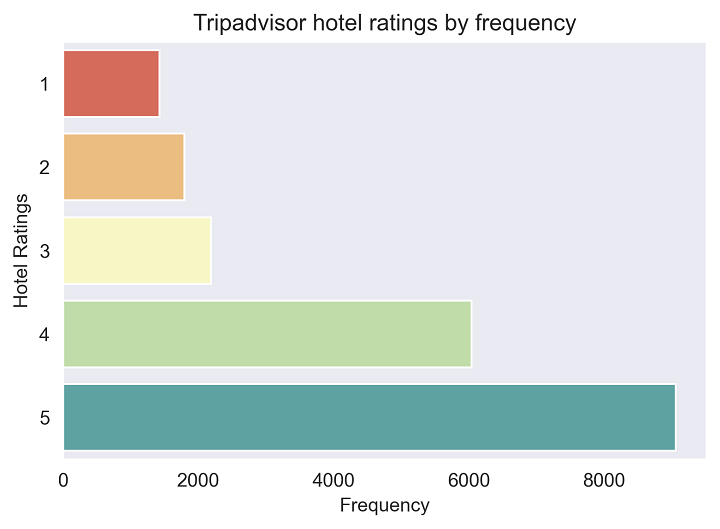
We can see how most hotel ratings fall between scores of 4 and 5. This shows that guests mainly have positive experiences, or at least that’s what they reported in the data. Now we can proceed to performing basic Natural Language Processing for the hotel reviews, using different libraries like re and NLTK.
Part 2: Performing basic NLP for the reviews
The first step is to clean our Tripadvisor reviews. This involves simple steps like removing punctuation, special characters, and numbers from each review.
#importing different NLP libraries:
import nltk
import re

#creating a subset for the reviews:
reviews = d1["Review"]
#creating a subset for the ratings:
ratings = d1["Rating"]

#transfroming all the words into lower case:
reviews = reviews.str.lower()

#removing special characters and numbers:
reviews = reviews.apply(lambda x : re.sub("[^a-z\s]","",x) )

#removing stopwords using NLTK:
from nltk.corpus import stopwords
stopwords = set(stopwords.words("english"))
reviews = reviews.apply(lambda x : " ".join(word for word in x.split() if word not in stopwords ))

#printing the first review to see if it worked:
print(reviews[0])
nice hotel expensive parking got good deal stay hotel anniversary arrived late evening took advice previous reviews valet parking check quick easy little disappointed nonexistent view room room clean nice size bed comfortable woke stiff neck high pillows soundproof like heard music room night morning loud bangs doors opening closing hear people talking hallway maybe noisy neighbors aveda bath products nice goldfish stay nice touch taken advantage staying longer location great walking distance shopping overall nice experience pay parking night
We can see that all punctuation has been removed, along with stop words and special characters. The next step is to represent this clean text numerically through a TF-IDF approach, which stands for Term Frequency and Inverse Document Frequency. Essentially, this approach counts the number of times a word appears in given document, while also considering the total number of documents in a dataset. This can be done relatively simple using this function from scikit-learn.
#loading the TfidfVectorizer from sklearn:
from sklearn.feature_extraction.text import TfidfVectorizer

#making the vectorizer:
vectorizer = TfidfVectorizer (max_features=2500, min_df=7, max_df=0.8)

#applying the vectorizer to the reviews:
processed_reviews = vectorizer.fit_transform(reviews).toarray()

#checking the length of the reviews variable:
len(processed_reviews)
20491
Now that we have vectorized the reviews, we need to generate a traning set and a testing set. The training set will be used to fine-tune the random forest model, while the testing set will be used to perform the ratings prediction. This can be done quite easily with another scikit-learn function:
#importing the test_split function:
from sklearn.model_selection import train_test_split

#making our subsets for the two variables
#the training set will be 80% of the data
#the testing set will be the remaining 20%:
x_train, x_test, y_train, y_test = train_test_split(processed_reviews, ratings, test_size=0.2, random_state=0)

#checking how many reviews fell into the testing set:
len(x_test)
16392
Part 3: Performing the random forest and making rating predictions
Before diving into the random forest, let’s define the algorithm. According to Donges (2020):
“Random forest is a flexible, easy to use machine learning algorithm that produces, even without hyper-parameter tuning, a great result most of the time. It is also one of the most used algorithms, because of its simplicity and diversity (it can be used for both classification and regression tasks).”
The algorithm is called a forest because it builds a series of decision trees, merging them together to get more accurate and stable predictions. Some of the most important model parameters will be highlighted as we go along. The first step is to perform the model on the training set:
#importing the random forest classifier from sklearn:
from sklearn.ensemble import RandomForestClassifier

#making the text classifier function
#the n_estimators refer to the number of trees we want to build
#the higher the n, the higher the power of the forest, but also a slower process
#we set the random_state to 0 so that it's replicable:
text_classifier = RandomForestClassifier(n_estimators=20, random_state=0)
text_classifier.fit(x_train, y_train)
RandomForestClassifier(n_estimators=20, random_state=0)
Now that we have made the basic model, we can do a prediction using the testing set. Additionally, we can use various accuracy measures to see how the model fits for each category:
#making the predictions:
predictions = text_classifier.predict(x_test)

#importing different accuracy measures:
from sklearn.metrics import classification_report, accuracy_score

#printing our results with these accuracy measures:
print(classification_report(y_test,predictions))
print(accuracy_score(y_test, predictions))
              precision    recall  f1-score   support

           1       0.61      0.49      0.54       285
           2       0.37      0.14      0.21       355
           3       0.36      0.09      0.15       471
           4       0.44      0.41      0.42      1203
           5       0.61      0.84      0.70      1785

    accuracy                           0.54      4099
   macro avg       0.48      0.40      0.41      4099
weighted avg       0.51      0.54      0.50      4099

0.5433032446938277
There’s a lot of information above, but the most important is the 54% accuracy for all our predictions. In the table above, there’s also accuracy information specific to each ratings class. For example, the random forest predicted 61% of all 1 and 5 star ratings. The model did not perform well for the middle ratings, i.e. scores from 2 to 4. In the last section we will try to improve this by simply adding more trees to the forest.
Part 4: Improving our model performance
To improve this model we could start by doing two different things:
- Perform a more exhaustive NLP and see if removing more words yields better results
- Add more trees to the random forest using the n_estimators parameter
Since this post is already quite long, we will go with the second option and see if this helps our model accuracy. This time we will visualize our classifier results using a nice plot from the Yellowbrick library.
#redoing the classification and stratifying the ratings:
x_train, x_test, y_train, y_test = train_test_split(processed_reviews, ratings, test_size=0.2,stratify=ratings)

#making a new random forest classifier with 80 trees:
model = RandomForestClassifier(n_estimators=80, random_state=0)

#importing the yellowbrick classifier:
from yellowbrick.classifier import ClassificationReport

#making the visualizer:
visualizer = ClassificationReport(model, support=True)

#fitting the visualizer to the training set:
visualizer.fit(x_train, y_train)

#evaluating the model on the test data:
visualizer.score(x_test, y_test)

#saving the output as an image file:
visualizer.show(outpath="post8_p2.png")

#showing the figure:
visualizer.show()
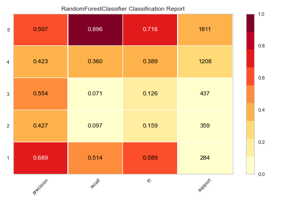
Conclusions
From the figure above, we can see a slight accuracy improvement by increasing the number of trees. One possible alternative is to perform a more robust NLP and filter out other words not included in the stopwords function. Another possibility could be combining the middle ratings. If we think about it, what is the qualitative difference between a rating of 2 or 3? What makes a hotel stay poor or simply average? The results suggest that the random forest has a better ratings prediction for the extremes, i.e. excellent or terrible hotel stays. This implies our language is clearer to this algorithm when we are either really upset or really happy. Fascinating!