
Using a Logit to Model Obesity Prevalence (R)
It’s time to post some actual research! So here is a bit of context to this post. My Bachelor’s degree was in Economics, but it was tough for me to follow the more theoretical classes. Things changed in my fourth year, when I took Econometrics. Just being able to model and apply what little I knew into friendly statistical programs felt great. So, once I finished those courses I wanted to keep going. I downloaded a nice data base from the Global Food Security Index(GFSI) and made a simple logit to model obesity. A few months later I was able to get it published in my university’s Economics Department. Ok, enough storytelling, let’s model!
Part 1: Data exploration
The database we’ll use is called “gsfi_logit.csv” and has already been cleaned and prepared. It contains the averages of each variable taken from the GFSI for the years 2012-2017. I didn’t use the yearly data in panel format because there were replicate observations for some of the variables. Therefore, we have averages for 112 countries (one country was removed as an outlier) during this short time period. The variables are coded as follow:
- obesity - represents an estimate of the national prevalence of obesity as a percentage of the total population.
- PPC - stands for GDP per capita.
- KCAL - an estimate of the average daily calorie intake for a person in a given country.
- div - an estimate of the dietary diversification, given as a percentage. Countries with higher values of div have diets comprised of more varied food groups.
- poverty - percentage of the population living below the global poverty line.
- consumption - the average spent on consumption as a proportion of a household’s income in a given country.
- popdens - is a country’s population density, taken from the World Bank.
- OECD - binary variable which takes the value of 1 if a country belongs to this group.
Time to explore the data:
#We will open the database and call it d1:
d1 <- read.csv("gsfi_logit.csv")
#feel free to perform the summary()
I developed a classification rule for the obesity variable. I took the mean value for all the countries (16.09) and made a binary variable. Those countries with obesity levels above the global mean were coded with 1, while those below the mean were given a 0:
#first we will create a null variable in our d1 database:
d1$obesd <- NULL

#now we generate the classification rule:
d1$obesd[d1$obesity>16.09]=1
d1$obesd[d1$obesity<=16.09]=0

#next we can code it as a factor:
d1$obesd <- factor(d1$obesd)

#to check how this obesity dummy is distributed we can use table():
table(d1$obesd)
##
##  0  1
## 48 64
#it is more or less balanced, 64 countries are above the global mean
Applying what we saw in the previous posts, we can do a nice graph to visualize possible relationships between our variables. We will perform a scatter plot of KCAL and GDP per capita, which also integrates our obesity variable:
#we first load ggplot2:
library(ggplot2)

#here is our basic plot and we shade our points according to obesity prevalence:
p1 <- ggplot(d1,aes(x=KCAL,y=PPC,color=obesity))+ geom_point(size=2)

#set up the color gradient with the most obese countries in red:
p2 <- p1 + scale_color_gradient(low = "steelblue", high = "red", name="Obesity prevalence(%)")

#we add a trend line, change the labels, and add a classic theme:
p2 + geom_smooth(method = lm,se=FALSE, col="darkorange")+
  ylab(c("GDP per capita"))+xlab(c("Average daily calorie intake per person"))+
  ggtitle(c("Obesity prevalence in countries by GDP and daily KCAL consumption"))+
  theme_classic()
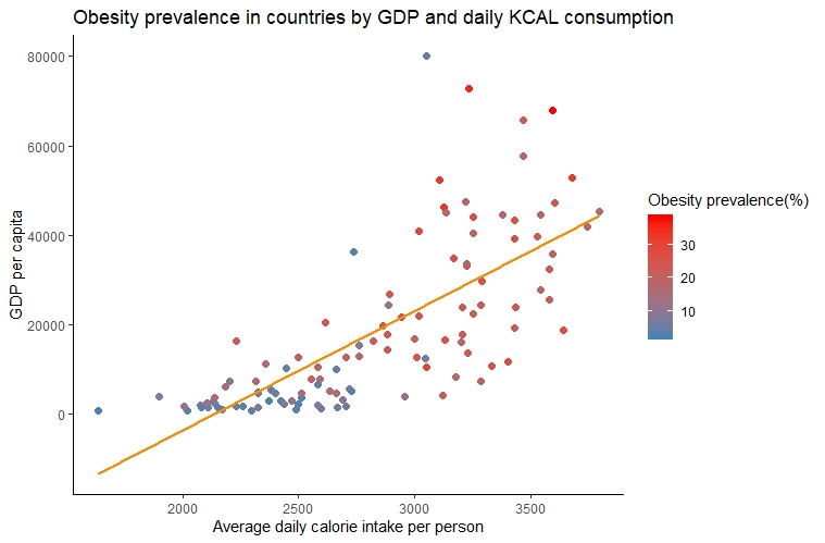
From our graph we can deduce the following:
- Countries with higher GDP per capita seem to have a higher average daily calorie intake per person.
- Obesity prevalence seems to have a positive relationship with the average daily calorie intake and possibly with a country’s GDP per capita.
Now it’s time to evaluate these theories using our logit model!
Part 2: Setting up our logit model
This part is relatively straigthforward. R has a built-in glm function which allows us to perform different models within the GLM framework. For a nice overview of GLM in R visit this course. We will start by recoding the OECD variable into a factor:
#we set our OECD variable as a factor:
d1$OECD <- factor(d1$OECD)

#now we perform our logit and save it as logit1:
logit1 <- glm(obesd ~ PPC + KCAL + div + poverty +
                consumption + popdens + OECD, data = d1,
              family = "binomial"(link=logit))

#the obesity dummy is the dependent ~ indepdendents
#dataset is d1, and the distribution is binomial
#the link functon is a logit

#we do a summary of our first logit:
summary(logit1)
##
## Call:
## glm(formula = obesd ~ PPC + KCAL + div + poverty + consumption +
##     popdens + OECD, family = binomial(link = logit), data = d1)
##
## Deviance Residuals:
##     Min       1Q   Median       3Q      Max
## -2.4075  -0.1955   0.1363   0.2592   2.0979
##
## Coefficients:
##               Estimate Std. Error z value Pr(>|z|)
## (Intercept) -1.185e+01  5.710e+00  -2.075   0.0380 *
## PPC         -3.590e-06  6.188e-05  -0.058   0.9537
## KCAL         3.290e-03  1.292e-03   2.546   0.0109 *
## div          1.122e-01  5.737e-02   1.955   0.0506 .
## poverty     -4.765e-02  2.595e-02  -1.836   0.0663 .
## consumption -1.737e-02  4.559e-02  -0.381   0.7032
## popdens     -1.717e-03  1.581e-03  -1.086   0.2775
## OECD1       -2.654e+00  1.413e+00  -1.879   0.0603 .
## ---
## Signif. codes:  0 '***' 0.001 '**' 0.01 '*' 0.05 '.' 0.1 ' ' 1
##
## (Dispersion parameter for binomial family taken to be 1)
##
##     Null deviance: 152.97  on 111  degrees of freedom
## Residual deviance:  51.53  on 104  degrees of freedom
## AIC: 67.53
##
## Number of Fisher Scoring iterations: 7
The summary of our first logit gives useful information on which regressors are statistically significant. In this case KCAL and div are the most significant, followed by the OECD dummy variable. We can use the anova function to determine if we should remove some of the other regressors based on the chi-squared criteria:
#here is the syntax for our deviance test:
anova(logit1, test="Chisq")
## Analysis of Deviance Table
##
## Model: binomial, link: logit
##
## Response: obesd
##
## Terms added sequentially (first to last)
##
##
##             Df Deviance Resid. Df Resid. Dev  Pr(>Chi)
## NULL                          111    152.971
## PPC          1   45.171       110    107.801 1.806e-11 ***
## KCAL         1   22.119       109     85.681 2.562e-06 ***
## div          1   22.576       108     63.106 2.020e-06 ***
## poverty      1    5.779       107     57.326   0.01621 *
## consumption  1    0.003       106     57.323   0.95684
## popdens      1    2.147       105     55.176   0.14285
## OECD         1    3.646       104     51.530   0.05621 .
## ---
## Signif. codes:  0 '***' 0.001 '**' 0.01 '*' 0.05 '.' 0.1 ' ' 1
According to this result we could consider removing consumption and population density. Let’s try to do so and see if we get better results:
#here we will generate our second logit:
logit2 <- glm(obesd ~ PPC + KCAL + div + poverty + OECD, data = d1,
              family = "binomial"(link=logit))
#this time we will just test the deviance:
anova(logit1,logit2)
## Analysis of Deviance Table
##
## Model 1: obesd ~ PPC + KCAL + div + poverty + consumption + popdens +
##     OECD
## Model 2: obesd ~ PPC + KCAL + div + poverty + OECD
##   Resid. Df Resid. Dev Df Deviance
## 1       104     51.530
## 2       106     54.709 -2  -3.1786
The second model does not show an improvement in terms of deviance. This is just one comparison criteria, but for now we’ll stick to the first model that includes all our regressors.
Part 3: Making predictions with our logit model
In this last section we will use our logit to make predictions. The first thing we will do is see how accurate our first logit model was in predicting countries with obesity prevalence above the global mean:
#we create a confusion matrix to see our model accuracy:
table(true=d1$obesd,pred=round(logit1$fitted.values))
##     pred
## true  0  1
##    0 42  6
##    1  3 61
From the diagonal of the matrix we can see that we correctly predicted about 92% of the cases. Of course, with more data we could generate a training and testing subset. For now, suppose we wanted to focus on predicting above average obesity levels for the OECD countries, one of the variables which was statistically significant:
#first we have to hold constant the means for our other variables and create a new df,
#we must keep the original names for each variable:
d2 <- with(d1, data.frame(PPC = mean(PPC), KCAL = mean(KCAL),
                                    div = mean(div),
                                    poverty = mean(poverty),
                                    consumption = mean(consumption),
                                    popdens = mean(popdens),
                                    OECD = factor(0:1)))

#now we generate the probailities:
d2$OECD_pred <- predict(logit1, newdata = d2, type = "response")
d2
##       PPC     KCAL      div  poverty consumption  popdens OECD OECD_pred
## 1 18622.8 2835.582 51.03839 25.99145    30.07974 209.7526    0 0.7347762
## 2 18622.8 2835.582 51.03839 25.99145    30.07974 209.7526    1 0.1631682
We can see from our prediction table that non-OECD countries show significantly higher probabilities of having obesity prevalence above the global mean! This result will be highligted in the following graph, its basic syntax was taken from here:
#for this graph we want to see how KCAL intake is related to
#obesity probabilites obtained, along with the OECD grouping:
d3 <- with(d1, data.frame(KCAL = rep(seq(from = 1600, to = 3800,
                                         length.out = 56),2), div= mean(div),
                                    PPC = mean(PPC),
                                    poverty = mean(poverty),
                                    consumption = mean(consumption),
                                    popdens = mean(popdens),
                                    OECD = factor(rep(0:1, each = 56))))

#now we will predict using the link scale:
d3 <- cbind(d3, predict(logit1, newdata = d3, type = "link",
                                    se = TRUE))
#now we include the residuals and Upper and Lower Confidence Levels:
d3 <- within(d3, {
  Probability <- plogis(fit)
  LCL <- plogis(fit - (1.96 * se.fit))
  UCL <- plogis(fit + (1.96 * se.fit))
})

#now we can generate our graph:
p3 <- ggplot(d3, aes(x = KCAL, y = Probability)) +
  geom_ribbon(aes(ymin = LCL, ymax = UCL, fill = OECD), alpha = 0.2) +
  geom_line(aes(colour = OECD), size = 1)

#extra customization for our plot:
p3 + ylab(c("Probability of having obesity levels above the global mean"))+
  xlab(c("Average daily calorie intake per person"))+
  scale_colour_manual(values=c("firebrick","midnightblue"),
                                         labels=c("Non-member", "Member country"))+
    scale_fill_manual(values=c("firebrick","midnightblue"),
                      labels=c("Non-member", "Member country"))+
  labs(caption = "Data extracted from GFSI/Economist Intellegence Unit")+
  theme(plot.caption = element_text(size = 7, face = "italic")) +
  geom_vline(xintercept = (median(d3$KCAL)), color="darkorange")
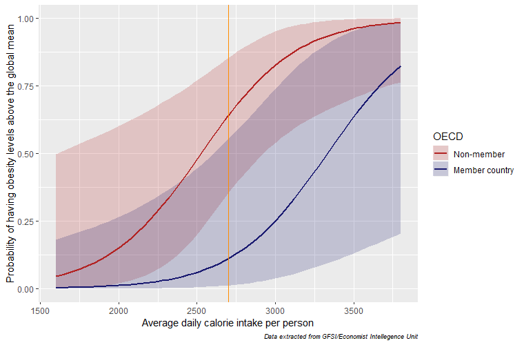
The shift is quite pronounced! From this plot we can see that for non-OECD countries, there is a higher probability of having above average obesity levels for any KCAL level, ceteris paribus. For example, notice the difference in the orange line of the probabilities for both groups at the median KCAL consumption!
What could this mean? One interpretation is that the quality of the calories consumed in non-OECD countries is poor compared to that of OECD countries. Lastly, we will do the same graph for the dietary diversification and see if the results hold. I removed the code so you can experiment with recreating it:
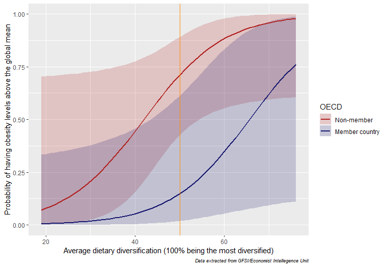
The results are very similar when it comes to the dietary diversification. Higher dietary diversification implies a higher probability for a country to have obesity levels above the global mean. Additionally, there is an even more pronounced difference between OECD countries and non-OECD countries.
Conclusions
Least developed countries have a higher probability of having obesity levels above the global mean, all things equal, for these two variables. While it is a short time period, this study seems to imply that the quantity of KCAL or degree of dietary diversification is not in itself a cause for higher obesity levels. The true issue probably lies in the quality of food accessible for least developed countries. These humble finding are still relevant in this global pandemic, as early studies have shown an alarming relationship between obesity and COVID-19 mortality. We must continue to study this global health issue, without losing sight of the inequalities present between countries.